In recent years, awareness of AI has become widespread, and it is being put to use by companies in many industries. There are expectations that AI will find use in manufacturing to solve various issues, such as improving productivity through automation.
In this blog post, we will explain the application of AI in the field of measurement control, using a sample program as an example.
Contents
What Is Artificial Intelligence (AI)?
There is no clear definition of AI, but it is generally recognized as a broad concept that includes technologies and processes that implement artificial systems that seem intelligent.
Machine learning and deep learning, which are often mentioned in association with AI, are a part of AI technology, as shown in Figure 1.
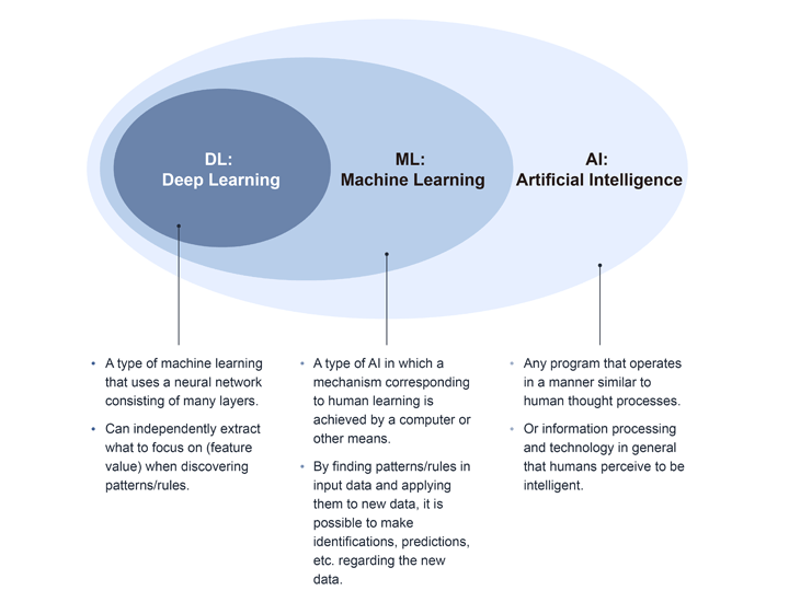 Figure 1: AI Conceptual Diagram
What Is Deep Learning?
Deep learning refers to the ability to automatically identify feature value, such as commonalities and regularities, by learning from large amounts of data.
Computers can now automatically determine feature value that previously required human input, as long as the well-prepared data is available. This has made it possible to carry out complex processes such as face recognition and noise removal, which were difficult to achieve with conventional machine learning.
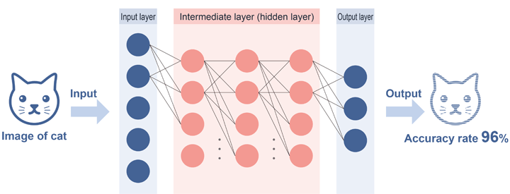 Figure 2: Deep Learning Conceptual Diagram
In this post, we will introduce unsupervised learning using autoencoders, which is the simplest form of deep learning, and a noise removal program using Python which has many libraries related to machine learning.
What Is an Autoencoder?
An autoencoder is a machine learning method that makes use of neural networks. It was developed to facilitate dimensionality reduction and feature extraction to eliminate unnecessary information, but in recent years it has been used as a generative model for anomaly detection and other applications.
In addition, although supervised learning can also be performed, autoencoder learning is basically unsupervised learning with the goal of outputting data that matches the input data.
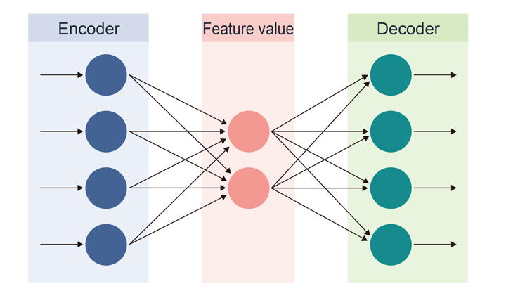 Figure 3: Autoencoder Conceptual Diagram
The autoencoder has the structure shown in the figure and learns by encoding/decoding from left to right. The circles in the figure are called nodes and the arrows are called edges.
Data is received from the nodes in the input layer, each edge is weighted individually, and the final value is the sum of those weights.
The function that performs dimensionality reduction and feature extraction in the first half of such a process is called the encoder, and the function that generates data based on the reduced dimensionality data in the second half is called the decoder.
The network of autoencoders is designed to reduce the dimensionality of the input data, return the data to its original form, and then output the data. It is also possible to employ encoder and decoder functions separately.
Noise Removal Program Using Autoencoders
In this post, we will use an example data set with pseudo-noise added to sine wave data sampled in the following configuration to create a Python program that implements unsupervised learning with autoencoders that will remove the added noise.
The source code for the sample programs in this article has been made open source. You can download it from the following link.
Sample program: Program to eliminate noise using autoencoder
Target device: DX-U1100P1-2E0211 edge AI computer + AI-1616L-LPE analog input card
Language used: Python 3.10
Libraries used: tensorflow, keras, etc.
First, execute the following command to install Python and the necessary libraries, etc. Also, some build tools are required to install Python, so be sure to install them as well.
# Install Python *Only when the Python environment is not installed
sudo apt update
sudo apt upgrade
sudo apt install build-essential libbz2-dev libdb-dev libreadline-dev libffi-dev libgdbm-dev liblzma-dev libncursesw5-dev libsqlite3-dev libssl-dev zlib1g-dev uuid-dev tk-dev
wget https://www.python.org/ftp/python/3.10.0/Python-3.10.0.tgz
tar -xf Python-3.10.0.tgz
cd Python-3.10.0/
./configure --enable-optimizations
make -j $(nproc)
sudo make altinstall

# Install library
pip install --upgrade pip
pip install tensorflow
pip install numpy pandas matplotlib scikit-learn opencv-python
Importing Libraries
First, import the required libraries.
import numpy as np
import pandas as pd
import matplotlib.pyplot as plt
from sklearn.preprocessing import MinMaxScaler
from keras.models import Sequential
from keras.layers import Dense
from IPython.display import display
Data Preprocessing
Pre-process the data set so that it can be properly processed for feature data extraction.
The prepared data will be converted to a one-dimensional array to generate data for training.
# Data window width
input_shape_num = 50

# Normalizing the dataset
scaler = MinMaxScaler()
# Calculating the transformation formula and perform data transformation
train_list = scaler.fit_transform(train_data[['Signal']], test_data[['Signal']])
test_list = scaler.transform(test_data[['Signal']])

# Flatten to one dimension array
train_list = train_list.flatten()
test_list = test_list.flatten()

# Creating partial time series
train_vec = []
test_vec = []
for i in range(len(train_list)-input_shape_num+1):
    train_vec.append(train_list[i:i+input_shape_num])
for i in range(len(test_list)-input_shape_num+1):
    test_vec.append(test_list[i:i+input_shape_num])
Model Definition
Next, the autoencoder model to be trained is defined using the keras Sequential model. The number of inputs to the model is compressed once and restored again to reduce overlearning and gradients while extracting features.
We will specify the information of the data to be trained in the layers of the Sequential model.
In this case, we will use the commonly-used Dense option (a fully-connected layer) from among the several keras layers.
Each parameter of Dense is explained below.
- units: Specifies the number of dimensions of the output.
- activation: Specifies the activation function to be used.
- input_shape: Passes a fixed array called a tuple. If there are multiple elements to be passed, they are represented as (0,1,2,...,n). In this case, the notation is (input_shape_num,) since there is only one element to be passed.
# Setting autoencoder
def init_autoencorder(input_shape_num):
    model = Sequential()
    # Encoding (number of output units = units, activation function = relu, number of inputs = input_shape_num)
    model.add(Dense(units=200, activation='relu',
              input_shape=(input_shape_num,)))
    # Decoding (Number of units to output = units, activation function = relu)
    model.add(Dense(units=100, activation='relu'))
    # Output layer (number of outputs = input_shape_num, activation function = sigmoid)
    model.add(Dense(input_shape_num, activation='sigmoid'))

    # Checking the model created
    model.summary()

    return model
Model Learning
Training is performed on the created autoencoder model.
First, the compile method must be used to set up the learning process.
Next, training data and other data must be specified in the fit method in order for the training to be executed.
The autoencoder can use either unsupervised or supervised learning, but since unsupervised learning is used in this case, training data is also specified for the teaching data (correct answer data).
Each parameter is explained below.
- optimizer: Specifies the optimization algorithm to be used.
- loss: Specifies the loss function (a function to calculate the deviation between the correct and predicted values of the model).
- metrics: Specifies the evaluation function (a function to measure the accuracy of the model).
# Running autoencoder
def run_auto_encoder(model, train_vec, batch_size, epochs):
    # Set learning conditions (optimization = adam method, loss function = mean squared error, evaluation function = accuracy rate of multi-class classification)
    model.compile(optimizer='adam', loss='mse', metrics=['acc'])

# Executing learning (training data = train_vec, teacher data = train_vec, number of gradient update samples = batch_size,
    hist = model.fit(x=train_vec, y=train_vec, batch_size=batch_size, number of training data iterations = epochs, progress display = progress bar, training data ratio)
                     epochs=epochs, verbose=1, validation_split=0.2)

    return hist
Learning Results
The generated model is applied to test noise data to evaluate the model.
# Evaluating the model on test data
pred_vec = model.predict(test_vec)
pred_vec = scaler.inverse_transform(pred_vec)
test_vec = scaler.inverse_transform(test_vec)

# Outputting test data to graph
plt.figure(figsize=(16, 2))
plt.plot(test_vec[:, 0], clor='blue', label='Test')
plt.plot(pred_vec[:, 0], color='orange', label='Filter')
plt.legend()
plt.show()
Now let’s confirm the results of the learning with the output graphs.
The orange line is the test data (data with noise added) and the blue line is the data to which the filter generated from the learning model is applied.
Generally, noise is removed and a pure sine wave is output.
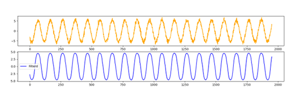 Figure 4: Applying Filters to Test Data
As you can see, Python makes it relatively easy to build noise removal programs using deep learning. This explanation is limited to simple sine wave data. However, by understanding the characteristics of each method and selecting appropriate parameters and data, it is possible to handle irregular signals that cannot be handled by conventional noise removal processing.
DX Series Edge AI Computers
Digital transformation (DX) enriches people’s lives by transforming with the evolution of digital technology. One of Contec’s solutions to achieve this is the DX series. The DX-U1100P1-2E0211 used in this noise reduction program is a general-purpose industrial edge AI computer that emphasizes practicality and is equipped with NVIDIA® Jetson Nano™ modules. It features a PCI Express slot, two Gigabit LAN ports, an HDMI port, two USB ports, general I/O ports, and an RTC (real-time calendar/clock) for flexible installation and environmentally-resistant performance.
The DX series aims to provide customers with new technologies such as AI, IoT, and 5G, which are indispensable for the realization of digital transformation, in a more familiar and easy-to-use manner.
Related Contents
See all blogs